Discover our
resources

A fun activity for a class with several robots: students train the robots to drive on a circuit, followed by a race. Through manipulation, students learn the principle of supervised learning and the importance of quality training data.

[Video content coming soon]

‍

‍

Introduction

Machine Learning is a branch of artificial intelligence whose aim is to enable computers to learn. A computer isn't intelligent; it simply performs tasks. In the form of programs, it is told what to do and how to do it. This is called programming.

Machine Learning deals with complex subjects where traditional programming finds its limits. Building a program that drives a car would be very complex, if not impossible. Machine Learning deals with this problem in a different way. Instead of describing what to do, the program will learn by itself how to drive by "observing" experiments.

Machine Learning: Enabling a program to learn tasks that have not been programmed.

Based on the experimental data that the learning algorithm takes as input, it will deduce an operating hypothesis on its own. It will use this hypothesis for new cases, and refine its experience over time.

There are three types of Machine Learning:

• Supervised learning
• Unsupervised learning
• Reinforcement Learning

Supervised learning is the most common type. It involves providing learning algorithms with a set of training data (Training Set) in the form of pairs (X, Y), with X the predictive variables (or input data), and Y the result of the observation (or decision). Based on the Training Set, the algorithm will find a mathematical function to transform (at best) X into Y. In other words, the algorithm will find a function F such that Y≈F(X) .

So, in situation X, it will know what decision Y should make.

Study situation and AlphAI robot training set

We now need to specify the X situations and Y decisions expected. 

The proposed case study is to move the robot in a red arena. The aim is for the robot to move on its own without ever touching the walls.

To do this, the robot can make the following decisions:

• Turn left 
• Go straight ahead 
• Turn right 

In order to make a decision, you need feedback in the form of data or a training set.

This is given by the sensors. The choice made here is to use the camera. From the camera's image area, two zones are extracted which will be called super pixels (see opposite). The amount of red in each super-pixel increases as the robot approaches the walls, due to the contrast between the white track and the red walls.

‍

‍

Activity 1. Indicate in the table below the result expected as a decision based on what is located in the superpixels.

‍

The simplified cases described above occur very rarely. To be able to make a decision in all possible cases, we need to know the numerical value of the red level. 

The camera image is 48*64 pixels in size. The position and geometry of the super-pixels is defined by the following figure:

‍

‍

Activity 2. Open the file get_values.py. Enter the path of the image forward_0.jpg and execute the code below to display the image in python.

from PIL import Image

import numpy as np

import matplotlib.pyplot as plt

def read_image(name):

    return np.array(Image.open(name, "r"))

img1=read_image("forward_0.jpg") #indicate image path

plt.imshow(img1)

plt.show()

You should obtain an image of the shape below, 48 pixels by 64 pixels in size, coded with the three RGB (Red Green Blue) colors.

"img1" is an array of pixels of size 48*64*3

The pixel array contains the 3 color levels Red Green Blue, coded between 0 and 255.

From this image, we'll need to extract the two super-pixels defined above and determine a method for obtaining the red level for each.

‍

‍

We will compare different techniques to obtain the best contrast between the red and white of each super-pixel:

• the average gray level of each super-pixel
• the average red level of each super-pixel
• the average green level of each super-pixel

‍

First, the image is transformed to grayscale using the rgb2gray function as follows:

def rgb2gray(rgb):

    return np.dot(rgb[...,:3], [0.299, 0.587, 0.144])

img2=rgb2gray(img1)

plt.imshow(img2, cmap="gray")

plt.show()

"img2" corresponds to the grayscale image. There is only one numerical value between 0 and 255 for each pixel. 0 corresponds to a white pixel and 255 to a black pixel. Super pixels are in the "lower" part of the image.

‍

‍

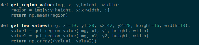
Activity 3. Write an average(img,x,y,height,width) function that takes as arguments an array of pixels "img" at one color level, the "x" and "y" coordinates of the top-left pixel of a super-pixel, the " height " and " width " of a super-pixel and returns the average color level of the super-pixel. 

‍

It is thus possible to retrieve two values with the two super-pixels defined above, using the code :

def get_two_values(img, x1=10, y1=28, x2=42, y2=28, height=16, width=13):

    value1 = average(img, x1, y1, height, width)

    value2 = average(img, x2, y2, height, width)

    return np.array((value1, value2))

The color level of the left super-pixel is value1, the color level of the right super-pixel is value2. It is thus possible to define a point with coordinates (value1, value2)

‍

‍

Activity 4. Execute the code to retrieve the value1 and value2 values from the grayscale image obtained previously.

The choice made in AlphAI software is to use the python mean function, which will calculate the mean value of the table.

‍

‍

‍

Activity 5. Apply the AlphAI software method and the greyscale method and complete with the values value1 and value2 in both cases.

Mean function

Grey Level

Forward_0

Forwad_1

Left_0

Left_1

Right_0

Right_1

Right_2

Test_0

Test_1

‍

‍

Activity 6. Place the points on the graph and identify the zones corresponding to the different decisions (turn left, go straight ahead, turn right). Conclude which method you think is the most appropriate for distinguishing the different decisions.

Right super-pixel intensity

Left super-pixel intensity

‍

At this stage, it would be possible to control the robot using conditional actions based on these super-pixel values. In what follows, we'll take a different approach. We're going to use a method known as theK-nearest neighbor algorithm.

‍

‍

The k-nearest neighbor algorithm, KNN

We're going to take a closer look at a well-known machine learning algorithm: the K Nearest Neighbours algorithm. This algorithm has the advantage of being very simple, and therefore provides a good basis for understanding supervised learning.

The idea is to use a large amount of data to "teach the machine" to solve a certain type of problem. The algorithm is particularly intuitive when the data is in the form of points in a 2-dimensional space, which can then be displayed on screen. So we're going to choose a configuration with just 2 sensor inputs, i.e. 2 "super-pixels" from the camera, to enable the robot to spot the walls and move around the arena without blocking. Initially, it will be up to us to tell the robot the associated action for each new piece of data (2 "super-pixels"), but then it will be able to move around on its own by choosing the majority action taken by the K nearest neighbors from the data entered during the training phase.

This supervised learning algorithm classifies data according to their proximity to the existing training data. The new data considers k neighbors, the k closest, to choose which classification to apply. With discrete data, such as points in a plane or in space, the nearest neighbors are selected using Euclidean distance, but other methods can be used in other situations, such as Manhattan distance if the data are placed on a grid or chessboard. The interest of this algorithm lies in the choice of k: too small and the algorithm becomes too sensitive to errors or missing data, too large and it considers data that should not be considered.

The operation of k-NN can be simplified by writing it in the following pseudo-code:

Start Algorithm

Input data :

• a data set D, corresponding to the training set created
• a function for calculating the distance between two points with coordinates [x1,y1] and [x2,y2]. d=x2-x12+y2-y12
• An integer k, representing the number of neighbors to be taken into account

For a new observation X whose decision Y we want to predict Do :

1. Calculate all distances between this observation X and the other observations in the dataset D
2. Select the K observations of dataset D closest to X using the distance calculation function d
3. Take the Y values of the k observations selected. Perform a regression and calculate the mean (or median) of the selected Y values. 
4. Return the value calculated in step 3 as the value predicted by K-NN for observation X.

End Algorithm

So you need to be able to calculate the distance between two points. In a two-dimensional graph, as in our example, this simply corresponds to the norm of the vector between the two points.

Activity 1. Write the function distance(point1, point2) which takes two points as arguments (point1=[x1,y1], point2=[x2,y2]) and returns the distance between these two points.

Activity 2. Complete the table below by determining the distance between the super-pixels of the previous images (forward_0.jpg, forward_1.jpg,...) and the two test images (test_0.jpg and test_1.jpg).

‍

Activity 3. Apply steps 3 and 4 of the K-NN algorithm, taking K=1,2,3 and 4, and deduce the decision to be made (go straight, turn left, turn right).

‍

‍

Robot drive

Preparing the working environment

• In the Parameters - > Load example configurations menu, select the "Supervised learning - KNN Camera" example configuration. 

Caution: For this scenario, to obtain the best possible contrast, place a white surface on the floor, and make sure you have uniform lighting across the surface of the arena.

‍

Training phase

Activity 1. Follow the protocol to complete the training phase

‍

You are now connected to the robot, and your screen should look like the image below. Its battery level should be displayed in the bottom right-hand corner (check that the robot is fully charged).

• As long as the robot has room to move, press go straight ahead. 

• If the robot approaches a wall, press turn on the spot to the left or right. 

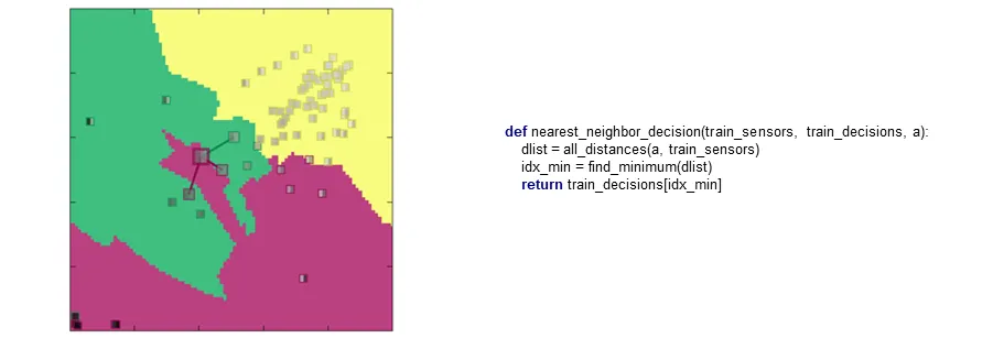
Each time an instruction is sent to the robot, a new point is added to the graph. The abscissa of this point corresponds to the value of the super-pixel on the left, and its ordinate corresponds to the value of the super-pixel on the right. The color of each point corresponds to the action chosen: yellow for going straight ahead, green for turning right and red for turning left. These points are the training data. This training phase is essential if the AI is to learn correctly. If the training data contains too many errors or approximations, the AI's behavior may not be satisfactory. 

Please note:

Pixels become darker as the robot approaches walls. Normally, if the left pixel is the darkest, turn right, and if the right pixel is the darkest, turn left. Once you've added a few points to the graphic, you can activate the background color in the visualization settings tab. This option colors each pixel of the graph with the color of the nearest data point.

When you have three clear areas on the graph, stop the training phase and reactivate the autonomy to move on to the test phase. Don't hesitate to move the robot by hand if an area of the graph contains too few dots.

‍

‍

Tests

If the robot is well trained, it will be able to avoid the edges on its own. If, on the other hand, the robot is poorly trained, or the arena's brightness is uneven, this will produce noise in the regions created, and the robot will perform more inappropriate actions.

Please note:

To obtain the best robot behavior, you need to test several values of k. To change this value, go to the "AI" tab and change the value of the "number of neighbors" parameter.

A good k value reduces the effect of noise and enables the robot to better manage unexplored regions.

Once the robot is well trained and the tests are running smoothly, you can move on to the activities.

‍

Activity 1. Compare the robot's behavior with k=1, k=3, k=10 and k=30. Then, based on what you see, try to determine the value of k that minimizes the effect of errors and gives the best robot behavior, i.e. the greatest distance covered without hitting a wall. The right value will depend on the number of data points, and the number of errors in that data.

‍

Activity 2. Now that you've understood the algorithm, try to train the robot with as little data as possible to enable it to turn without banging into walls. 

‍

Start by making a theoretical version by drawing the areas you'd like to obtain on your graph. Which points need to be placed to achieve this? Test these points with the robot after entering them into the software. Was your theoretical model applicable in reality, or did you have to make any modifications? What are the limitations of this method for a robot like this?

Tip: You can move the robot by hand to select the points you want to teach it.

Note: We managed to teach the robot to move around the arena without hitting the walls with just 3 points.

To find out more :

‍

Activity 3. If you have time left and want to experiment, switch algorithms and see how the robot behaves differently from KNN. What other algorithm would you suggest for faster learning? And what other algorithm do you think would enable learning of more complex tasks, such as kicking a green ball or recognizing commands communicated with hand signals?

‍

‍

Program the K-nearest neighbor algorithm

1. Stop the robot and reactivate the "Stand-alone" button.

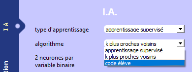
2. In the AI tab, select Algorithm: student code , this will open a new window asking you to name the file. 

3. After giving it a name, the file appears in Windows Explorer: open it in your favorite code editor (Spyder, for example).

This code presents 3 existing functions: init, learn and take_decision. These functions will be called by the main software. Only the take_decision function is important for this tutorial.

4. Note that when you disconnect, a simulated mini-robot appears in the bottom right-hand corner. If you wish, you can do the questions below with this mini-robot and return to the real robot at the end of the test; but you can also do the whole test while connected to the real robot: as you prefer!

‍

‍

PROGRAM THE ROBOT DIRECTLY

Before programming an artificial intelligence, let's start by understanding the principle of the take_decision function. You'll be able to modify this function to change the robot's behavior: after each modification, save your code and click on the "Reset AI" button. This step must be repeated for each code modification: save, then reload the code.

The function has the following prototype:

take_decisionsensors:listint

The sensors input is the state of the robot's sensors, i.e. in our case a list of two values sensors[0] and sensors[1], which are the intensity of what the robot sees to its left and right. Its output is the number of the chosen action.

1. Add the print(sensors) instruction inside the function. Save, click "Reset AI" in the software, and start the robot. The sensors value is now displayed in the console (click on the icon in the taskbar to display the console). What is the approximate sensors value when the robot is facing a wall? when it's not facing a wall? when there's a wall to its left or right?

‍

2. For now, the function returns 0. What value must be returned for the robot to go straight ahead? (Try it out)

‍

3. Use the variable x to program consistent robot behavior: "If there's no wall, I go straight; if there's a wall, I turn."

‍

‍

ALGORITHM PROGRAMMING

Distance calculation

If you haven't already done so in the previous activity, program a new distance function that takes as arguments two points a and b, which are arrays of two elements each containing their coordinates, and returns the Euclidean distance of these two points. The prototype of the function is as follows:

distancea:list, b:listfloat

With a=x1, y1 and b=x2, y2

As a reminder, the Euclidean distance between these two points is: d=x2-x12+y2-y12.

The square root can be used in Python by importing the math (or numpy) library at the top of the :

import math

and is written as follows :

y = math.sqrt(x)

The square operator can be made as follows:

y = x**2

4. Program the new distance function. Then, to test it, write at the bottom of the :

# compute distance

a = [0, 0]
b = [1, 2]
print("distance", distance(a, b))

Save, load the code with "Reset AI" and note the result displayed in the console below:

‍

Calculating all distances

Now that you have a method for calculating a distance, write a new function all_distances that calculates all the distances from a point to the variable train_sensors, which are the drive input data. This function will take as argument a new point x which is a list of two elements as before, and return an array containing all these distances. Its prototype is :

all_distances(a:list[float], train_sensors:list[list[float]])→list[float]

With a=x0, y0 and train_sensors=x1, y1, x2, y2, ..., xn, yn The train_sensors array being of length n.

‍

5. Program all_distances, then test with the following code at the bottom of the file:

# compute all distances

a = [0.4, 0.6]

train_sensors = [[0, 0], [0, 1], [1, 0]]

distance_list = all_distances(a, train_sensors)

print('distances to data', distance_list)

Reload the code and copy your result:

‍

Find the smallest element in an array

Create a function called find_minimum, taking an array as its only argument and returning the index of the first smallest element. Its prototype is :

find_minimum(dlist:listfloat)→int

6. Program and test find_minimum with the following code:

# minimum in a list

idx_min = find_minimum(distance_list)

print('index of minimum', idx_min)

Note the result:

‍

The nearest neighbor

Now that we have all the functions we need, we can create the nearest_neighbor_decision function, which takes the drive data and the current camera input as arguments, and returns the command to be sent to the robot. Its prototype is :

nearest_neighbor_decision(train_sensors:list[listfloat],train_decisions:list[int],a:list[float])→int

As before, a=x0, y0 and train_sensors=x1, y1, x2, y2, ..., xn, yn and train_decisions = d1,...,dn where each di is the decision made for point xi, yi in the train_sensors array. 

To realize the function, calculate the distances, find the shortest and return the associated command using train_decisions.

‍

7. Program and test nearest_neighbors_decision with the following code:

# KNN

a = [0.4, 0.6]

train_sensors = [[0, 0], [0, 1], [1, 0]]

train_decisions = [1, 2, 0]

decision = nearest_neighbor_decision(train_sensors, train_decisions, a)

print('KNN', decision)

Copy the result:

‍

‍

USING YOUR ALGORITHM WITH THE ROBOT 

Congratulations, you've programmed the K-nearest neighbor algorithm yourself in the case of K=1. Now you just need to use it in the program to train the robot.

To do this, copy the lines below to program the take_decision function to make the right decisions, but also learn to remember the train_sensors and train_decisions training data that will be created as you go along in the main program:

train_sensors = train_decisions = None

def learn(X_train, y_train):
global train_sensors, train_decisions
train_sensors, train_decisions = X_train, y_train
loss = 0
return loss

def take_decision(sensors):
if train_sensors is None:
return 0
return nearest_neigbor_decision(train_sensors, train_decisions, sensors)

 And now you can train your robot!

1. Reload your code

1. Deactivate the robot's autonomy by clicking on the icon

1. ,
2. Steer the robot by clicking on the arrows on the right of the screen. Turn when the robot is close to the walls, otherwise go straight ahead. 

The train_sensors and train_decisions tables are filled in automatically by the software each time you click an arrow.

4. After a short training period, reactivate autonomy

4. The robot navigates the arena alone. Does it avoid the walls on its own?

‍

‍

Further information

The algorithm you've written uses the nearest neighbor to make its decision. Modify your code so that it takes into account the majority of decisions made between a number k>1, k∈N. The difficulty lies in modifying the function that finds the minimum. It must now find k and not just 1.

‍

‍

Review and feedback

‍

In programming, the list of accessible program functions is called an API, for Application Programming Interface. It is used by programmers to find out how to interact with the program. You'll find the API for the alphai python module here: https: //drive.google.com/file/d/1C4ovPW_eH5KFz5Y9JvSrzLhtmdOpcp6-/view